4.3 Notation
Mathematicians use several notations for expressing derivatives.
Myron supports two: Leibnitz notation and LaPlace notation.
Leibnitz notation combines a derivand and a derivator into what is
essentially a binary operator: “derive this with respect to
that”. Leibnitz notation is often used to produce standalone
expressions; everything that is required to define the derivative is
specified in the notation. Thus
 ⅆx^2ⅆx
can be simplified to
ⅆx^2ⅆx
can be simplified to
 2⋅x.
2⋅x.
Leibnitz notation is sometimes treated as if the derivand and the derivator are separate terms.
Thus the equation
 ⅆx:1÷ⅆy:1=1 can be transformed to
  ⅆx:1=ⅆy:1. To support this
usage, Myron provides decoupled derivatives, in contrast to the combined,
or coupled derivative in the previous paragraph. Decoupled derivatives that appear as operands
of a divide operator act like the coupled derivative they resemble.
ⅆx:1=ⅆy:1. To support this
usage, Myron provides decoupled derivatives, in contrast to the combined,
or coupled derivative in the previous paragraph. Decoupled derivatives that appear as operands
of a divide operator act like the coupled derivative they resemble.
Sometimes the derivand is not an expression and is instead a function
reference.
 ⅆf(x)ⅆx
does not contain enough information to be transformed using
derivation, but it does contain enough information to be transformed
to LaPlace notation. That is,
ⅆf(x)ⅆx
does not contain enough information to be transformed using
derivation, but it does contain enough information to be transformed
to LaPlace notation. That is,
 .{ⅆf(x)ⅆx.}
and special Simplify produce
.{ⅆf(x)ⅆx.}
and special Simplify produce
 f’(x). These two expressions are related; special Simplify on the latter reproduces the former.
Laplace notation extends to antiderivatives. Replacing the previous example with
integration, special simplification of  .{∫f(x) ⅆx.} produces
 f'{-1}(x)+ĉ.
LaPlace notation for higher-order derivatives and anti-derivatives uses a higher tick count.
Nested derivatives like  f’’’(x) transform (after three special simplifications) to
 ⅆⅆⅆf(x)ⅆxⅆxⅆx. This in turn can be transformed to the Leibnitz form
 ⅆf(x)ⅆx:3. Similarly, the antiderivative of
  f'{-3}(x)
transforms to
f'{-3}(x)
transforms to 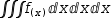 ∫∫∫f(x) ⅆx ⅆx ⅆx.
LaPlace notation is useful when the elaboration of a function is not
relevant. For example, Newton's method for finding a root can be
expressed in part using the recursive relation
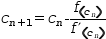 c_(n+1)=c_n-f(c_n)÷f’(c_n). To use this function in a concrete way, f and f’ must be bound to
global definitions, say,
c_(n+1)=c_n-f(c_n)÷f’(c_n). To use this function in a concrete way, f and f’ must be bound to
global definitions, say,
 f(x)→sin x
and
f(x)→sin x
and
 f’(x)→cos x. (The second function can be produced symbolically by converting a
copy of the first to a differential function and simplifying the right
side.) By choosing this
f’(x)→cos x. (The second function can be produced symbolically by converting a
copy of the first to a differential function and simplifying the right
side.) By choosing this  f(x), Newton's method will find the root
of
f(x), Newton's method will find the root
of  sin x, i.e., the point at which the sin curve crosses the x-axis.
Then the recursive relation must be expressed as a function.
sin x, i.e., the point at which the sin curve crosses the x-axis.
Then the recursive relation must be expressed as a function.
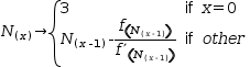 N(x)→x=0?3:N(x-1)-f(N(x-1))÷f’(N(x-1))
Here,
x is the number of iterations, descending recursively to 0,
where iteration 0 returns the approximation 3.
 N(2)
N(2) evaluates to 3.141592653300477
and
 N(3)
N(3)
evaluates to 3.141592653589793.
N(3) differs from
 ℼ
ℼ
in the tenth decimal place.